Probing Physics in Motion Diffusion Models Against Their Own Estimate
Do motion diffusion models know more physics than they show? I recorded every layer of three models and compared them, fairly, with each model's own running guess of the finished motion. Almost everything the layers know is already in the guess.
arXiv preprint, 2026
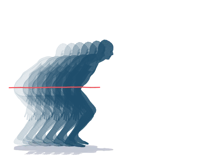
Ask a text-to-motion model for “a person walks forward slowly and carefully” and look closely at what comes back. Most samples are fine. In some, partway through a step, both feet leave the floor and the whole body glides along a few centimetres up for half a second, as if it were on a moving walkway, before it sets down again. Nothing pulls it back to the ground, because nothing in the model enforces the ground.
That is the normal state of affairs. Most text-to-motion models are kinematic: they output joint positions and rotations directly, with no physics simulator anywhere, so whatever physics they get right was picked up from motion capture and is never enforced. Their best-known failures are physical ones. Bodies hover, feet slide while they are planted, jumps don't fall the way they should. The usual fixes work from the outside, for example by pushing samples through a physics simulator[2].
Meanwhile, papers on video generators have been reporting something intriguing. Physical properties can be decoded from the generator's internal activations better than from its output, which one paper sums up as models that “know more than they show”[3]. Others localise physical quantities inside the transformer[4] and use probes on the denoising features to prune bad samples early[5]. If the same were true of motion models, it would be useful: a signal inside the model could flag a floating sample long before compute is spent finishing it.
So that is what I set out to show in this paper[1]: that a motion diffusion model, too, knows more than it shows, and that this knowledge can stop failing samples early. It is not what I found. In this article I want to walk through what I measured, why the usual comparison is misleading, and the one small place where the layers really are ahead. I'll use a single jump as the running example, the one in the clip above. The code snippets are simplified Python sketches of the ideas rather than the code I ran.
If you would rather watch first, here is the paper as a six-minute narrated overview:
The paper in six minutes
Narrated overview, 6:25, with captions in the video
- How a Motion Is Generated
- Measuring Physics From Joints
- What “Knowing More” Would Mean
- Physics Shows Up Early
- The Advantage Disappears
- The Exception: How Fast a Jump Falls
- What Actually Goes Wrong
- Can the Guess Warn Us Early?
- A Detour Into Video
- Lessons
- Limitations and What's Next
- Citation
How a Motion Is Generated
The models in this study are diffusion models. MDM[6], which I used in two versions (its 50-step and its original 1000-step checkpoint), and MotionDiffuse[7] were both trained on HumanML3D[8], and both make six seconds of motion at a time: 120 frames at 20 frames per second. A sample starts as pure noise. At every step the model looks at the current noisy motion and the text and predicts what the finished motion will look like, and the sampler then takes a small step from the noise towards that prediction.
That prediction, the model's running guess of the finished motion, is the hero of this article. In the paper it is called the clean-motion estimate. It is a complete, playable motion at every step. MDM predicts it directly, and MotionDiffuse predicts the noise, from which the guess follows by a fixed formula. Here is the guess for our jump at four moments, played side by side:
Watch a jump take shape
The same sample of the 50-step MDM, its guess at four points of generation, in sync
This is the first surprise, and it shapes everything after it. A fifth of the way into generation the jump is already decided. If the model held its physics somewhere inside and only revealed it late, the guess at 20% would look vague. It doesn't. You can step through the same sample more slowly here:
Step through it yourself
One recorded sample of the 50-step MDM, “a person jumps forward”: the model's guess at four points of generation. Each picture shows the same half-second, every second frame from take-off to landing.
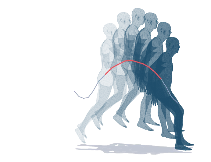
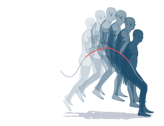
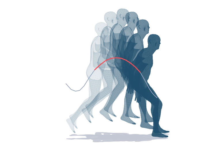
9.5 m/s²how fast the body falls in the guess at 20% of the way
Real gravity: 9.81 m/s²
To study what the model knows, I recorded everything along the way. For every sample, at six steps spread evenly from the first to the last, I kept the guess, the noisy input, and the output of every one of the transformer's eight layers at every fourth frame. Roughly:
def sample_and_record(model, text, steps=50):
    x = torch.randn(120, 263)                  # 6 s of motion at 20 fps, as pure noise
    keep = evenly_spaced(steps, 6)             # the steps we record
    record = {}
    for k, t in enumerate(model.timesteps(steps)):
        guess, layers = model(x, t, text, return_layers=True)   # MDM predicts the clean motion
        if k in keep:
            record[k] = (guess, layers)        # the guess, and every layer that computed it
        x = model.step(x, guess, t)            # one small step towards the guess
    return x, record                           # the finished motion, and its history
The main prompt set has 250 prompts: 64 that I wrote to cover walking, jumping, balancing and everyday actions, and 186 captions from the HumanML3D test set. Each prompt was sampled four times, with three seeds per model, which gives 6,000 recorded motions from the two MDM checkpoints and 3,000 from MotionDiffuse. Jumps turned out to be rare in that set, so I later added a jump-heavy set of 245 prompts (one caption from every HumanML3D test motion described as a jump, hop, leap or skip, plus 14 of my own), which adds 2,940 motions per model.
Measuring Physics From Joints
A nice thing about motion, compared with video, is that physics can be computed exactly from the output. There is no need for a simulator or a human judge: given the joint positions, a handful of formulas say whether the body is balanced, whether it is in the air, and how fast it falls. And because the guess is a full motion at every step, the same formulas work on the guess too.
Everything starts from the centre of mass, a weighted average of the body's segments using standard mass fractions. A foot joint counts as in contact when it is close to the floor and nearly still. For balance I used the extrapolated centre of mass[9]: the centre of mass pushed forward by its velocity, which says where the body is heading, not just where it is. The signed distance from that point to the area under the feet is the dynamic balance margin. It is negative through most of every normal step, which is how walking works (you are always catching a fall), so I treat it as a continuous number rather than a failure flag.
For flight, a frame is airborne when every foot joint is off the floor and no knee, wrist or the pelvis is near it either. Over each airborne stretch of at least 0.2 seconds I fit a parabola to the height of the centre of mass. A body in free flight falls at 9.81 m/s², and that test needs no calibration: if the parabola says 9.5, the jump falls about right. If it says less than 2 m/s², the body is off the ground and unsupported but barely coming down. That is floating.
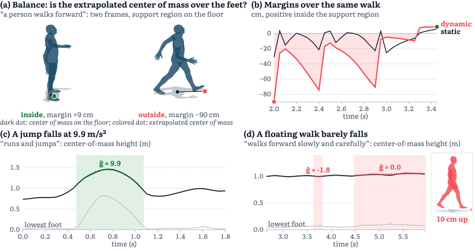
The gravity test fits in a few lines:
def fall_rates(com_height, airborne, fps=20):
    """A parabola fitted to the centre of mass over each airborne stretch of at least 0.2 s."""
    out = []
    for start, end in stretches(airborne, min_len=int(0.2 * fps)):
        t = np.arange(start, end) / fps
        a2, a1, a0 = np.polyfit(t, com_height[start:end], 2)
        out.append((start, end, -2 * a2))      # a real jump falls at 9.81 m/s²
    return out

def floating(rates):
    return [(s, e) for s, e, g in rates if g < 2.0]   # off the ground, but barely falling
One confession belongs here. My first definition of “airborne” only looked at the feet. It counted crawling and cartwheels as flight, and it fitted parabolas to bodies that were hovering, which made the 1000-step model's jumps look as if they fell far too slowly (a median of 3.75 m/s² in one seed). Once hovering was separated out, that effect vanished. Labels deserve the same suspicion as results.
What “Knowing More” Would Mean
The standard way to ask what a model knows is a probe: a small readout, often linear, trained to predict a property from the model's internal activations. If a probe on a layer predicts the finished motion's balance better than the balance computed from the model's own guess, it is tempting to say the model knows how balanced the motion will be and fails to show it.
Here is the catch. The guess is computed from those same activations. In MDM the last layer is mapped to the guess by a fixed linear projection, and every earlier layer feeds the next one. So everything the guess contains about balance has passed through the layers. Information can't appear out of nowhere along the way (this is the data-processing inequality), which means the guess can never hold more about the outcome than the layers and the noisy input together. The reverse can happen, of course, but a probe that beats a readout of the guess doesn't show that. It shows that the information is easier for that particular probe to use in the layer. The guess might still contain all of it, in a form that needs a nonlinear readout or a computed quantity like the balance margin.
There is a name for “how much of the information a given kind of readout can use”: usable information[10]. Unlike ordinary information it can grow with processing, which is exactly how a probe on a layer can beat a weak readout of the guess. The question that actually bears on hidden knowledge is what the layer adds to the guess[11]. So instead of pitting the two against each other, I trained two readers for every target and step: one that sees only the guess, and one that sees the guess and a layer. Both are tuned the same way, and the gap between them is what the layer knows that the guess does not show.
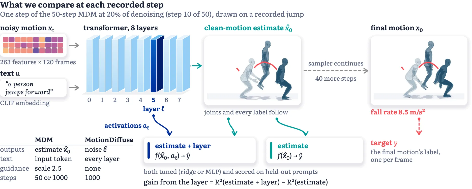
Getting this comparison right took three precautions, and each of them mattered somewhere. The readers must be equally flexible and equally well tuned, so I used ridge regression and a family of small MLPs for every input, picked by validation error on held-out prompts. The test must hold within a prompt: physics varies a lot between prompts, and a reader could score well just by recognising which prompt it is looking at, so I also score after removing each prompt's average (and, with seeds pooled, each prompt's average at each frame). And there must be enough training data, because, as you'll see, with too little data the comparison can flip. The combined reader is also allowed to fall back to the guess alone, so that a bigger input can't lose just by being harder to fit:
def gain_from_layer(guess, layer, target, prompts):
    folds = group_kfold(prompts, k=5)          # no test prompt is ever seen in training
    alone = tuned_readout([guess], target, folds)             # ridge or MLP, whichever validates better
    both = tuned_readout([guess, layer], target, folds,
                         may_fall_back_to=alone)              # free to ignore the layer
    return r2(both) - r2(alone)                # what the layer knows that the guess does not show
Physics Shows Up Early
The first result matches the clip. A fifth of the way through generation, linear probes on the layers already recover the finished motion's dynamic balance with an R² of 0.84, and whether a frame is in flight with an AUC of 0.97, on the 50-step model. Those numbers hold across seeds and on prompts the probes never saw, and they are about the same on my hand-written prompts (0.835) and on test captions (0.839). The 1000-step model is less readable at the same point (0.70 for balance).
Taken at face value, the standard comparison also suggests hidden knowledge. For balance and flight, the best layer beats both the label computed from the guess and a linear probe on the guess. For dynamic balance on the 50-step model, the layer is ahead of the computed label by 0.045 to 0.065 in R² depending on the seed. That is the kind of gap that gets written up as a model knowing more than it shows. Switch the chart below between the two comparisons:
How much more do the layers know?
Show as a table
The Advantage Disappears
Read with the same care, the guess keeps up. With seeds pooled and every reader tuned on held-out prompts, the tuned readout of the guess beats the tuned readout of the layer for both balance measures, by 0.015 to 0.029 in R² on the two MDM checkpoints and by 0.12 and 0.18 on MotionDiffuse. For flight it ties or leads. And adding the layer to the guess gains nothing: for balance and flight, on all three models, the gain is at most 0.01, and every interval covers zero or lies below it, both across prompts and within prompt and frame. I checked every layer, not just the chosen one. None adds more than 0.007.
A null result is only worth something if the method could have found a positive one, so I ran a positive control. I took the part of the target that the guess's reader gets wrong, added noise so that its best linear use would raise R² by just 0.005, 0.01 or 0.02, hid it in the layer's activations along a random direction, and ran the whole procedure again without changing anything. For dynamic balance even the smallest planted signal was found: a gain of +0.013, against +0.000 for the real layer. So the protocol can see a gain of that size, and the real layer doesn't have one.
Two details show where the usual comparison goes wrong. First, the kind of reader matters. Restricted to linear readers, the layer does add a little (up to 0.02 on MDM), because part of what the guess shows needs a nonlinear readout. Second, on MDM the input matters even more than the reader: from its 263 raw numbers per frame alone, the tuned guess only ties the tuned layer, and the physics labels computed from it add about 0.02 for balance. Give the reader of the guess the balance margin itself, and it no longer needs to work it out.
Small training sets can flip the answer
Before the main study I ran a pilot with 64 prompts and a single held-out set of 12. It pointed the other way: the one-number label computed from the guess beat the best layer on dynamic balance, 0.832 against 0.814. The amount of training data explains it. A one-feature label barely depends on how many prompts you train on, while a 512-feature layer probe needs between 52 and 100 training prompts to overtake it. With tuned readers the same thing happens: at 25 training prompts the computed label beats every trained reader (0.783, against 0.757 for the tuned guess and 0.617 for the tuned layer), and from 50 prompts on the guess leads the layer at every size. The gain from adding the layer stays at zero throughout. A comparison at one training size can favour either side. Only a lead that persists as data grows tells you something about the model. Video probing benchmarks are of a similar size, which is worth keeping in mind.
The Exception: How Fast a Jump Falls
There is one target where the layers really do know more, and it took me a while to see it, because my original gravity label mixed two questions. In the main data, most airborne frames lie in stretches that barely fall at all, so a score for “flight gravity” mostly measures whether a body floats or falls, which the guess shows early and well. Splitting the label into “floats or falls” and the fall rate of the stretches that do fall, and measuring the latter on the jump-heavy prompts, changed the picture for that one quantity.
On the jump prompts of the 50-step model, adding a layer raises the R² for the fall rate from 0.35 to 0.43, a gain of +0.077 (95% interval 0.051 to 0.107). It replicates on the 1000-step model (+0.076), and every layer from 3 to 7 adds 0.06 to 0.08. I tried hard to explain it away. It isn't just the layer knowing where the jump is: in 92% of the falling frames the guess at 20% is airborne too, and there the layer still adds +0.069. It isn't a weak reading of the guess's timing, because the reader already gets the guess's own fitted fall rate, and a reader that sees all 30 recorded frames at once still leaves the layer ahead. It isn't the text: giving the reader the prompt's own text embedding doesn't help on held-out prompts. And it isn't label noise, because on real motion capture the gravity label is precise enough to allow an R² of 0.81 to 0.91.
The one thing the layers know first: how fast a jump falls
R² for the finished jump's fall rate, on held-out jump prompts; tuned readouts, seeds pooled
Show as a table
But the gain doesn't last. At 40% of the way the layer still adds 0.043; by 60% no layer adds more than 0.02, and at 80% the interval covers zero, because the guess's reader improves faster than the layer's. That has to happen eventually, since the finished motion is the last guess. What the measurement adds is the size and the duration: about 0.08 in R², for about two fifths of the trajectory. At a fifth of the steps, MDM's middle and late layers carry information about how fast a jump will fall that its guess does not yet show in any form I could read. It is a real, if small, case of a model knowing more than it shows.
On MotionDiffuse the same gain is smaller and less stable: +0.025 at 20%, holding within prompt but not within prompt and frame, and zero in one of two refits. Matching the noise level doesn't close the gap either. MotionDiffuse's noise schedule is linear where MDM's is cosine, so “20% of the way” is far noisier for it (a signal-to-noise ratio of 0.002, against 0.10 for MDM). At its 60% point the noise is between MDM's at 20% and 40%, and there its gain is only +0.007, against MDM's +0.077 and +0.043 at those two points.
What Actually Goes Wrong
Along the way the measurements answered a simpler question too: what goes wrong physically in these motions? Not the jumps, mostly. When MDM's bodies leave the ground and fall, they fall at close to the right rate in the median: 9.54 to 9.75 m/s² for the 50-step model on my jump prompts and 9.13 to 9.22 m/s² for the 1000-step model, a little slower than real jumps in the processed training data (10.33 m/s²). Individual jumps do spread widely around those medians.
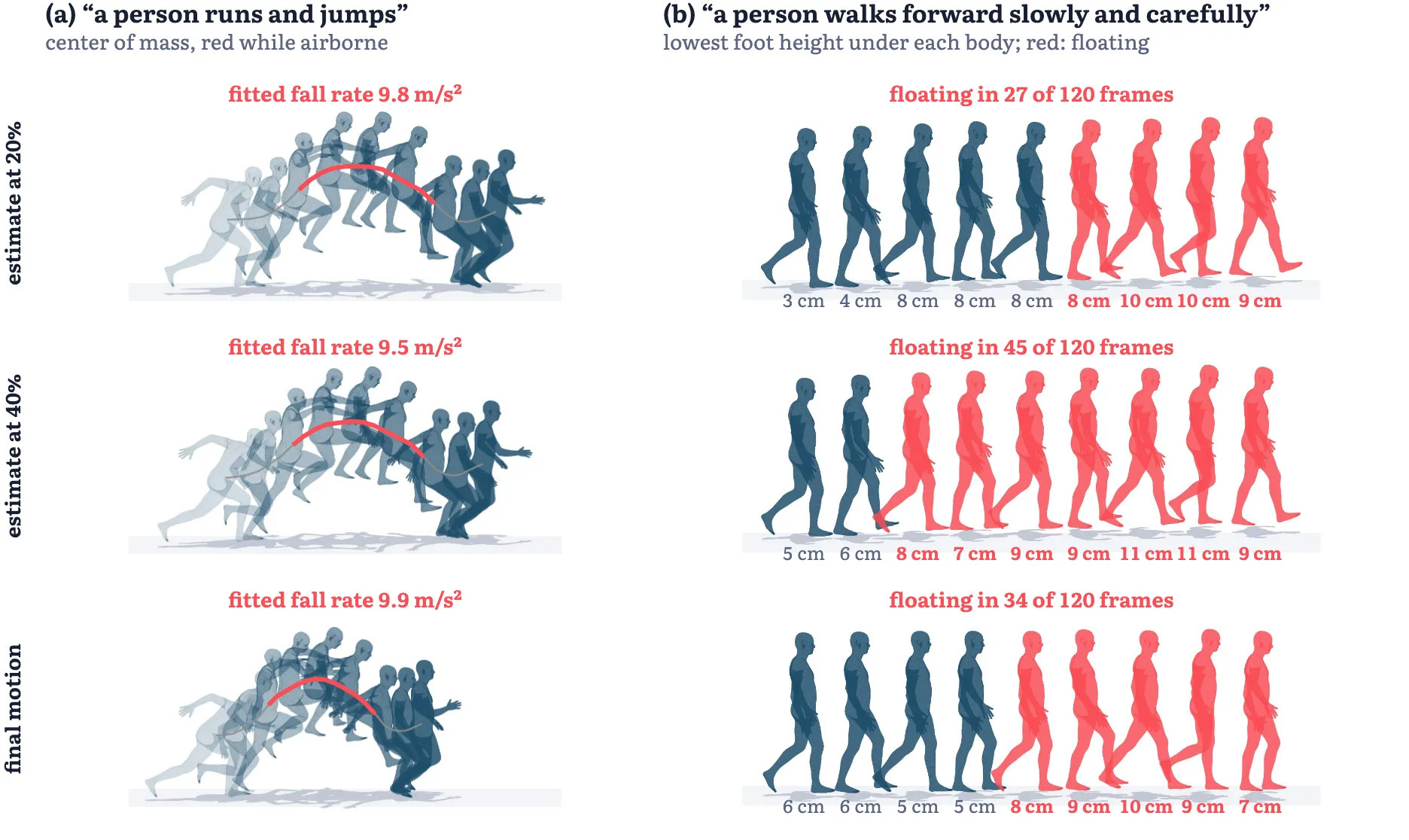
The common failure is floating, the walkway glide from the start of this article. On HumanML3D test captions, 3.8 to 4.7% of the 50-step model's frames lie in floating stretches, against 8.6 to 9.7% for the 1000-step model, so the original checkpoint floats about twice as often, in every seed and under every threshold I tried. Some of it is implied by the prompt: a person “walking on a balance beam” is generated without a beam and floats in nearly every sample. On real motion capture, the same labels flag floating in 0.09% of frames.
A slow walk that floats
“A person walks forward slowly and carefully”, 50-step MDM; red while floating
Here are the same two motions as the paper's opening figure, frame by frame:
Can the Guess Warn Us Early?
The practical hope behind all this was early warning: catch a sample that will float partway through, restart it, and save the compute of finishing it. The guess turns out to be a good enough warning signal on its own, with no training at all. If the guess at 20% of the way shows any floating, the finished motion floats in 80% of cases on the 50-step model and 82% on the 1000-step model, and this simple rule catches 59% and 47% of all floating samples. At 40% of the way the precision rises to 88% and 84%. Trained readouts of the guess, of a layer, or of both do about as well as the rule, so the layers don't help here either.
The payoff, though, is small. Checking a finished motion for floating costs almost nothing, so the baseline to beat is simply to finish every sample, check it, and try again if it floats. Against that, aborting at 20% when the guess floats saves 3.4 to 6.7% of the compute on the 50-step model and 4.3 to 9.9% on the 1000-step model, at the same rate of delivered floating. Even a perfect detector would save only 6.7 to 14.9% and 11.9 to 22.5%.
Catching floating motions early saves little
Floating motions delivered against compute (1 = one full sample), as the number of tries grows
The reason is in the numbers. Floating affects only 9 to 18% of samples, and it is concentrated in particular prompts. After 20 tries, 2.6 to 3.7% of delivered motions still float, from prompts like the balance beam that float in nearly every sample. The paper works out the ceiling in closed form, and the simulation agrees with it to within 0.0015.
A Detour Into Video
The video papers that started this make a related claim about inputs: that plausibility is absent from the video generator's clean latent (the compressed form of the video it works on), because a linear probe on that latent scores at chance, so the transformer must be building it[3]. I wanted to know whether “a linear probe is at chance” really means “absent”.
I encoded the IntPhys development set[12] with the Wan 2.1[13] video encoder and tried to read plausibility from the latent: in each pair of matched videos, which one is physically possible? The fully averaged latent is at chance, as reported, and so is every readout that is linear in the latent, between 50 and 55%. One fixed, training-free change makes the difference: take the size of the frame-to-frame change on a coarse 4 × 4 grid, and read that linearly. It reaches 78% pairwise accuracy on its own, and 80% together with the grid features. It beats every one of 1,000 label-shuffled runs, and it isn't a global artefact of how the impossible videos are made: overall frame-to-frame change is almost the same in possible and impossible videos, and training-free “largest change” scores are at chance.
There is a simple reason the averaged baseline fails. An average over time can't tell apart videos whose frames are rearranged in time, and impossible events like an object vanishing or teleporting are mostly changes over time. So plausibility isn't linearly decodable from the clean latent, but it is present there, and one simple transform exposes it. That doesn't show the transformer adds nothing. It does mean that a probe at chance is weak evidence that a property is absent.
Lessons
Compare a model with its own output first
A diffusion model's guess of the finished sample is computed from its activations, so it is the natural baseline for any claim about what the activations know. Read it as carefully as the layers, with the same readers tuned the same way, and report what the layer adds to it. In my case that one change made almost all of the hidden knowledge disappear.
Check that the method could have found something
A null result needs a positive control. Planting a small, known signal in the layer and recovering it is what turns “the layer adds nothing” from an absence of evidence into evidence, and it also showed me which scores could not see small gains (a pooled AUC near its ceiling barely moves).
Watch how much data the comparison has
With a few hundred examples, a 512-feature probe and a one-number baseline can trade places. My pilot study reached the opposite conclusion from the full study for exactly this reason. A lead that persists as the training set grows is the only kind I would trust now.
Look at what a label is made of
My gravity score looked like a measure of how fast bodies fall. It was mostly a measure of whether they float, which the guess shows early. The one genuine case of the layers knowing more only appeared after the label was split.
Before calling something absent, try a simple transform
In the video latent, every linear readout was at chance and the signal was still there, one absolute value away. “Not linearly decodable” and “not present” are different claims.
Limitations and What's Next
- Two families of model. I studied kinematic transformer diffusion models trained on HumanML3D: MDM at two checkpoints and MotionDiffuse. Models with other training data or designs, such as token-based generators, may behave differently.
- Heuristic labels. Contact heights, the support rule and the 2 m/s² floating cut-off are thresholds. On real motion capture they flag almost no floating and recover the fall rate of real jumps closely, but I checked one dataset.
- Relative to the readers I tried. “The layers add nothing” holds for ridge and tuned MLPs on one frame at a time and a small temporal network. A stronger reader could change it, and it is the layer side that a stronger reader could still raise.
- Correlation, not use. I don't know which computation in the layers carries the fall rate, or whether steering along it would change how fast generated jumps fall.
- Simulated early warning. The savings come from replaying recorded samples, with exactly the information an online run would see.
The next test I would most like to see is the same comparison inside a video generator, along its own sampling path, with a physics label measured from the generated video (the fall rate of a tracked object, say) and the model's decoded preview as the baseline. The same question also matters for the motion planners inside physics-based character controllers and humanoid robots: if the planner's own guess already shows that a motion is off balance, the controller underneath knows when to step in.
Citation
Saeed Ghorbani. Probing Physics in Motion Diffusion Models Against Their Own Estimate. arXiv:2611.24423, 2026.
@article{ghorbani2026probing,
  title   = {Probing Physics in Motion Diffusion Models Against Their Own Estimate},
  author  = {Ghorbani, Saeed},
  journal = {arXiv preprint arXiv:2611.24423},
  year    = {2026}
}
References
- S. Ghorbani. Probing Physics in Motion Diffusion Models Against Their Own Estimate. arXiv:2611.24423, 2026.
- Y. Yuan, J. Song, U. Iqbal, A. Vahdat, J. Kautz. PhysDiff: Physics-Guided Human Motion Diffusion Model. ICCV 2023.
- P. Esmati, S. Nath, K. Hofmann, D. Nowrouzezahrai, S. E. Kahou, M. Mirmehdi. The Invisible Hand of Physics: When Video Diffusion Models Know More Than They Show. arXiv:2606.05328, 2026.
- J. Kneifl, J. Skalski, B. Twardowski, K. Deja. Does Physics Live in the Activations? Localizing Physical Quantities in Video Diffusion Models. arXiv:2610.03154, 2026.
- C. Tang, L. Zhong, F. Ding. Seeking Physics in Diffusion Noise. arXiv:2603.14294, 2026.
- G. Tevet, S. Raab, B. Gordon, Y. Shafir, D. Cohen-Or, A. H. Bermano. Human Motion Diffusion Model. ICLR 2023.
- M. Zhang, Z. Cai, L. Pan, F. Hong, X. Guo, L. Yang, Z. Liu. MotionDiffuse: Text-Driven Human Motion Generation with Diffusion Model. arXiv:2208.15001, 2022.
- C. Guo, S. Zou, X. Zuo, S. Wang, W. Ji, X. Li, L. Cheng. Generating Diverse and Natural 3D Human Motions from Text. CVPR 2022.
- A. L. Hof, M. G. J. Gazendam, W. E. Sinke. The Condition for Dynamic Stability. Journal of Biomechanics, 2005.
- Y. Xu, S. Zhao, J. Song, R. Stewart, S. Ermon. A Theory of Usable Information Under Computational Constraints. ICLR 2020.
- J. Hewitt, K. Ethayarajh, P. Liang, C. D. Manning. Conditional Probing: Measuring Usable Information Beyond a Baseline. EMNLP 2021.
- R. Riochet, M. Ynocente Castro, M. Bernard, A. Lerer, R. Fergus, V. Izard, E. Dupoux. IntPhys 2019: A Benchmark for Visual Intuitive Physics Understanding. IEEE TPAMI, 2021.
- Team Wan et al. Wan: Open and Advanced Large-Scale Video Generative Models. arXiv:2503.20314, 2025.